How to use Monte Carlo Simulation with Brownian Motion

In this article, we will demonstrate how to implement a Monte Carlo simulation for stock prices using Geometric Brownian Motion (GBM) in a simple way, explaining the basic underlying logic to understand how to perform it in a correct way.

In mathematical finance, an asset is often modeled as following a Geometric Brownian Motion, meaning it adheres to a stochastic differential equation (SDE).
GBM assumes that the price moves up and down randomly, but it also has a general trend of increasing or decreasing over time. It does this by considering two things: how fast the price changes on average (called the "drift") and how much the price randomly jumps up or down (called the "volatility"). It assumes that the logarithmic returns of these assets follow a normal distribution.

For this example, we will gather the price of Apple stock, and we will perform the GBM Monte Carlo simulation for the same time scope.
Then, we will plot the simulations alongside the original evolution trend of the stock.

Two Approaches to Modeling GBM

1. Black-Scholes Formula Approach:

   The Black-Scholes formula suggests that the returns of an asset follow a log-normal distribution. By applying the corresponding mathematics, we derive the following standard formula for the asset price dynamics:

   S(t) = S(0) * exp((μ - 0.5 * σ²) * t + σ * W(t))

   Where: μ is the drift (annualized average return of the stock), and σ is the volatility (standard deviation of returns).
   The term -0.5 * σ² in a correction for the "drag" effect in returns, that is fixed in the formula.

   Intuitive Explanation of the Correction: The correction -0.5 * σ² addresses the drag problem that arises in asset returns due to the multiplicative nature of returns.
   For example if an asset has returns of +50% and -50% its value will be (1.5 * 0.5) * asset, reducing to 0.75 times the value of the asset after a round, and eventually converging to zero. By applying this corrections this effect is mitigated.

   Now below we can use the following code and see the result

   GBM Monte Carlo Simulation for Apple Stock (2021-2024)

   For this demonstration, we will simulate the Apple stock price from 2021 to 2024 using Python. This example will provide a clear illustration of how to apply these models in practice.

   import numpy as np
   import pandas as pd
   import yfinance as yf
   import matplotlib.pyplot as plt
   from matplotlib.lines import Line2D
   
   apple = yf.download('AAPL', '2021-1-1','2024-1-1')
   apple.columns = apple.columns.levels[0]
   price = apple.Close
   returns = price.pct_change().dropna()
   
   t = len(returns)
   dt=1
   mu = returns.mean()
   sigma = returns.std()
   geom_mu = ((returns+1).prod())**(1/t)-1
   simulations = 1000
   S0 = price[0]
   
   def GBMpaths(mu, sigma, W):
       return np.exp((mu-0.5*sigma**2)*dt+sigma*np.sqrt(dt)*W)
   
   Ws = np.random.standard_normal(size=(simulations,t))
   GBM_matrix = GBMpaths(mu,sigma,Ws)
   GBM_matrix = np.insert(GBM_matrix,0,S0,axis=1).cumprod(axis=1)
   
   xAxis = range(0,t+1)
   
   fig, ax = plt.subplots(figsize=(12, 5.5)) 
   for n,i  in enumerate(range(1,simulations)):
       plt.plot(xAxis,GBM_matrix[n],color='grey', linewidth=0.1)
   plt.plot(xAxis,price,color='red',linewidth=1)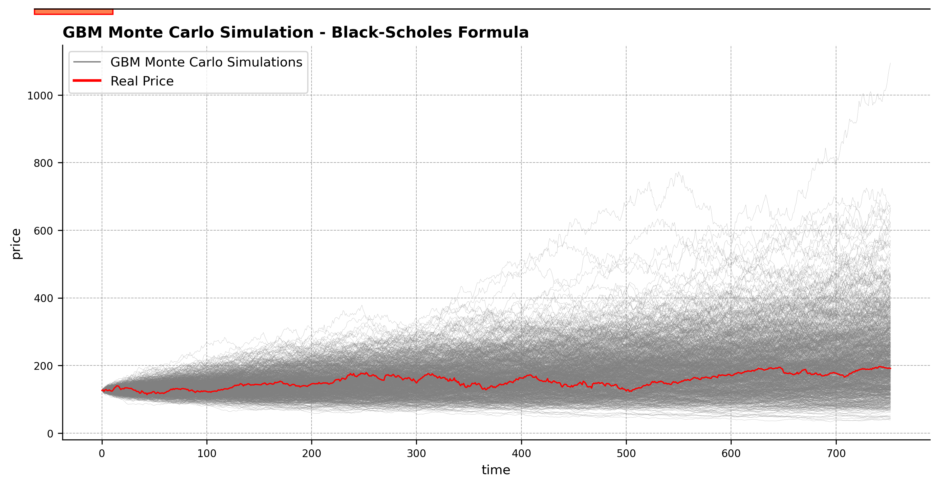

   
2. Log Transformation Approach:

   In this approach, as we assumed that the asset's returns follow a log-normal distribution, we just apply a log transformation to the returns. After applying the log transformation, we can model the transformed data using standard Brownian Motion. This method leads to the same underlying model but through a different mathematical lens.

   GBM Monte Carlo Simulation for Apple Stock (2021-2024) - Log Transform

   This is the code when we will apply a log-transform and apply a simple Browninan motion to these models.

   log_returns = np.log(returns+1)
   mu_log = log_returns.mean()
   sigma_log = log_returns.std()
   
   def BMpaths(mu, sigma, W):
       return mu + sigma * W
   
   BM_matrix = BMpaths(mu_log, sigma_log, Ws)
   BM_matrix  = S0*np.exp(BM_matrix.cumsum(axis=1))
   BM_matrix = np.insert(BM_matrix,0,S0,axis=1)
   
   fig, ax = plt.subplots(figsize=(12, 5.5)) 
   
   xAxis = range(0,t+1)
   for n,i  in enumerate(range(1,simulations)):
       plt.plot(xAxis,BM_matrix[n],color='grey', linewidth=0.1)
   plt.plot(xAxis,price,color='red',linewidth=1)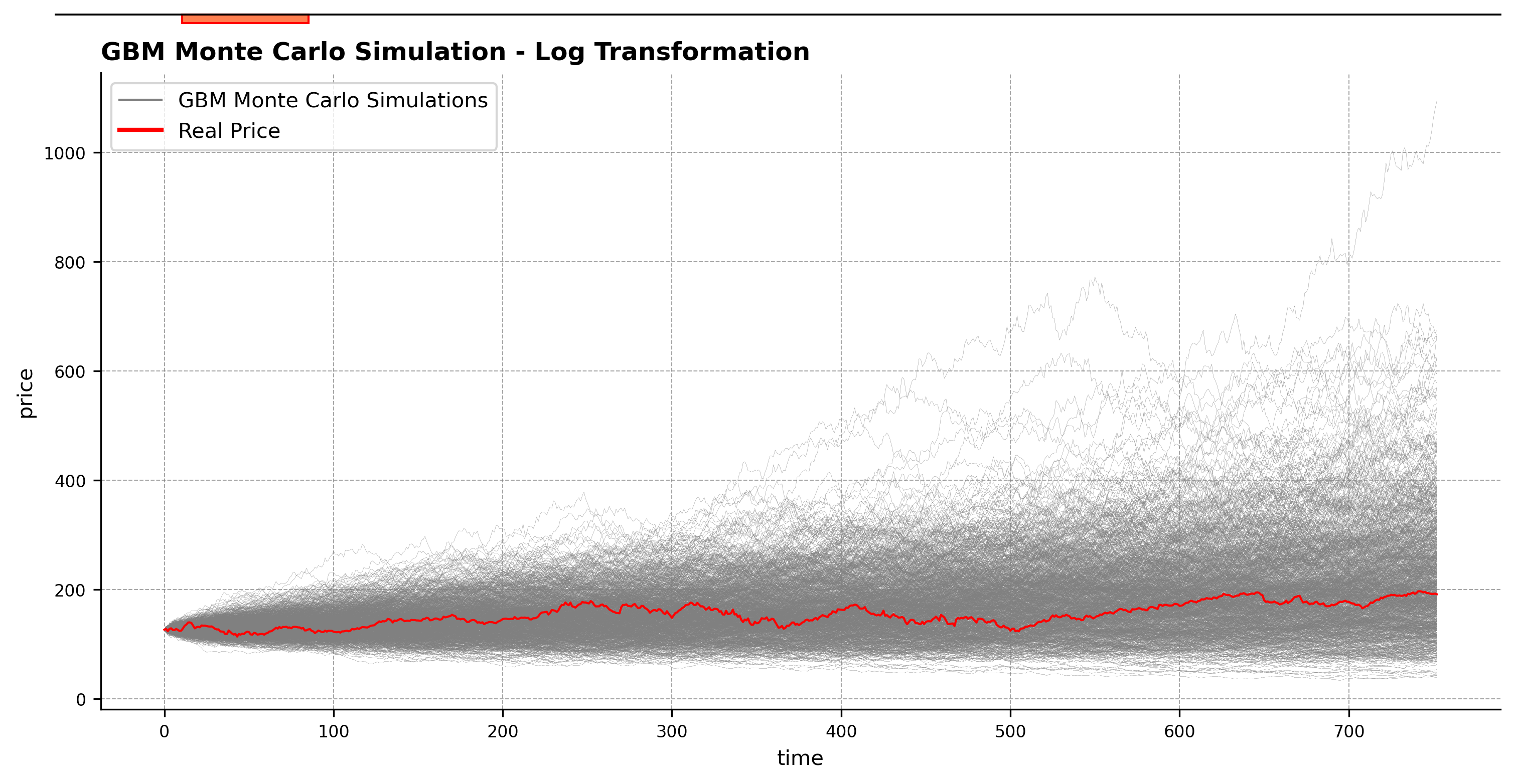
   

   

Comparing Both Results

Comparing both charts, we can see that the results are practically identical (with a perfect normal distribution for the log-returns; they converge to the same exact result), verifying the two methods mentioned above for performing correct Geometric Brownian Motion Monte Carlo simulations.